Real Analog: Chapter 9

Back to Chapter 8

Chapter 9 Materials

• Lecture Material:
  • Lecture 24 PowerPoint Slides: Introduction to state-variable modeling, simulating system response using MATLAB
  • Lecture 24 Video
• Chapter 9 Video:
  • Lab 9 Video 1: State Variable Models: The step response of the state variables of a series RLC circuit are measured. The measurements are compared to the simulated response obtained by using MATLAB.
• Chapter 9 Complete PDF
  • Lab 9.3.1
    • Worksheet 9.3.1
  • Lab 9.3.2
    • Worksheet 9.3.2
• Exercise Solutions: Chapter 9 exercise solutions
• Homework: Chapter 9 homework problems

In our analysis approach of dynamic systems so far, we have defined variables which describe the energy in the circuit energy storage elements (voltages across capacitors and currents through inductors). We then used KVL and KCL to write differential equations describing the circuit, in terms of those variables. The resulting equations were then combined into a single differential equation governing the parameter in which we were interested (the input-output equation for the system); this equation was solved to determine the response of the circuit. This approach is useful for low-order systems, such as the first or second order systems we have examined so far, but it becomes cumbersome for higher-order systems. An alternate modeling approach, state variable (or state space) modeling, has a number of advantages over the approach we have been using to date, especially for higher-order systems.

In this chapter, we will provide a very brief introduction to the topic of state variable modeling¹⁾. The brief presentation provided here is intended simply to introduce the reader to the basic concepts of state variable models, since they are a natural – and relatively painless – extension of the analysis approach we have used in Chapters 7 and 8. Introduction to state variable models at this stage also allows the reader to perform numerical simulations of system responses. Numerical simulations are computer-generated solutions to the differential equations governing the system. Most numerical approaches to the solution of differential equations require the equations to be in state variable form²⁾.

State variable models of dynamic systems consist of several first order differential equations, in several different variables. (These variables are called the state variables.) The state variables for a system must completely describe the energy contained in all the energy storage elements in the system, so natural choices of state variables for electrical circuits are the voltages across capacitors and the currents through inductors. If there are $N$ state variables required to describe the circuit, the state variable model is created by applying KVL and KCL to obtain N first-order differential equations in these $N$ variables. Please notice that this approach is exactly the approach we have used in Chapter 8 to determine the differential equation governing a second order circuit – we are simply eliminating the step in which the individual equations are combined into a single, higher-order differential equation in a single unknown. Since the mathematics associated with combining the individual equations can be tedious, state variable models are actually easier to create than input-output equations!

A brief description of state variable models is provided in section 9.1 of this chapter. An example of the state variable model for a third order system is provided to illustrate development of the model. Section 9.2 provides information relative to numerical simulation of a state variable model using MATLAB, and section 9.3 provides Octave syntax to perform the same processes³⁾.

If desired, this chapter can be skipped without loss of continuity.

• Define state variables for electrical circuits
• Write differential equations governing electrical circuits in state variable form
• Use MATLAB and/or Octave to simulate the impulse response of an electrical circuit
• Use MATLAB and/or Octave to simulate the step response of an electrical circuit
• Use MATLAB and/or Octave to plot the state trajectory of an electrical circuit

As their name implies, state variable models are based on the concept of a system’s state. The state of a system is the minimum amount of information necessary to completely characterize the system at some instant in time. More specifically, if we know the state at any time, and the input to the system for all subsequent times, we can determine the output of the system at any subsequent time⁴⁾. It turns out that the system’s state uniquely determines the energy in all the system’s energy storage elements and vice-versa. If the energy in any of the energy storage elements changes, the system’s state changes.

The state variables are the smallest set of variables which completely describe the state (or the energy storage) of the system. The choice of state variables is not unique, but one possible choice of state variable is those variables which describe the energy stored in all of the independent energy storage elements in the system. For example, in electrical circuits, inductors store energy as current and capacitors store energy as voltage. If we choose as state variables the currents in inductors and the voltages across the capacitors, we will have created a legitimate set of state variables for the circuit.

Since the state variables are independent, they can be visualized as a set of orthogonal axes defining a space. The space defined by the state variables is called state space of the system. If the system is described by $N$ state variables, the state space will be N-dimensional. The state of the system at any given time can be visualized as a point in the state space.

In general, as the system responds to some input, the system’s state will change over time. Since the state of the system is a point in state space, the change in the system’s state can be visualized as tracing a path over time in the state space. This path is called the state trajectory.

State variable models, as mentioned previously, represent an $N^{th}$ order system as N first order differential equations in $N$ unknowns. (The unknowns are the state variables.) For linear, lumped-parameter, time invariant systems, these equations will take the form:

$$\dot{x}_1 (t) = a_{11}x_1(t)+a_{12}x_2(t)+ \dots + a_{1N}x_N(t)+b_1u(t) \\ \dot{x}_2(t) = a_{21}x_1(t)+a_{22}x_2(t)+ \dots + a_{2N}x_N(t)+b_2u(t) \\ \cdot \\ \cdot \\ \cdot \\ \dot{x}_n = a_{N1}x_1(t)+ a_{N2}x_2(t)+ \dots + a_{NN}x_N(t)+b_Nu(t) \\ (Eq. 9.1)$$

Where $x_1(t)$, $x_2(t)$, $\dots$, $x_N(t)$ are the system and $u(t)$ is the input to the system. The overdot notation denotes differentiation with respect to time; $\dot{x}_k(t)=\frac{dx_k(t)}{dt}$. (We will assume that no derivatives of the input are applied to the system – this is a special case which we will avoid in this introductory chapter.)

It turns out that, if all system states are known, we can determine any other parameter in the system. In fact, any other parameter in the system can be written as a linear combination of the states and the input. Thus, we can write the system output as:

$$y(t)=c_1x_1(t)+c_2x_2(t) \dots + c_Nx_N(t)+du(t) (Eq. 9.2)$$

Equations (9.1) and (9.2) are commonly written in matrix form as:

$$\underline{\dot{x}}(t) = A \underline{x}(t)+\underline{b}u(t) (Eq. 9.3)$$

$$y(t)= \underline{c} \underline{x}(t)+du(t) (Eq. 9.4)$$

In equation (9.3), the vector $\underline{x}(t)$ is an $Nx1$ column vector containing the system state variables. The matrix $A$ is a square $NxN$ matrix, and the vector $\underline{b}$ is an $Nx1$ column vector. The vector $\underline{\dot{x}}(t)$ is an $Nx1$ column vector containing the derivatives of the state variables as a function of time. In equation (9.4), the vector $\underline{c}$ is a $1xN$ row vector, and $d$ is a scalar. Equation (9.3) provides the state equations for the system, and equation (9.4) is called the output equation of the system.

It is possible to define more than one output in a system⁵⁾. To define multiple outputs, we simply create a vector of outputs, each row of which is an equation of the form of equation (9.2). For example, if we define P outputs, the set of output equations becomes:

$$y_1=c_{11}x_1+c_{12}x_2+ \dots + c_{1N}x_N+d_1u \\ y_2=c_{21}x_1+c_{22}x_2+ \dots + c_{2N}x_N+d_2u \\ \cdot \\ \cdot \\ \cdot \\ y_P=c_{P1}x_1+c_{P2}x_2+ \dots + c_{PN}x_N+d_Pu \\ (Eq. 9.5)$$

In the case of multiple outputs, we modify our matrix expression of equation (9.4) to:

$$\underline{y}(t)=C \underline{x}(t) + \underline{d}u(t) (Eq. 9.6)$$

Where $\underline{y}(t)$ is a Px1 column vector containing the outputs, C is a PxN matrix, and $\underline{d}$ is a Px1 column vector.

Creation of the state variable model for an electrical circuit is probably best described by example. Examples of creation of state variable models for both second and third order circuits are provided in the examples below. Please notice that the creation of a third order state variable model is not significantly more difficult that creation of a second order state variable model. Creation of a third order input-output equation is, however, generally considerably more difficult than creation of a second order input-output model. (Try, for example, creating an input-output relation for the circuit of example 9.2 below.)

A series RLC circuit is shown below. Appropriate state variables are the current through the inductor and the voltage across the capacitor, as shown.

Applying KVL around the circuit loop, we obtain:

$$u=x_1+0.5 \dot{x}_1+x_2$$

Applying KCL at the node between the inductor and capacitor results in:

$$x_1=0.5 \dot{x}_2$$

Rearranging the above equations and placing them in matrix form results in:

$$\begin{bmatrix} \dot{x}_1 \\ \dot{x}_2 \end{bmatrix} = \begin{bmatrix} -2 & -2 \\[0.3em] 2 & 0 \\[0.3em] \end{bmatrix} \begin{bmatrix} x_1 \\ x_2 \end{bmatrix} + \begin{bmatrix} 2 \\ 0 \\ \end{bmatrix} u(t)$$

Since the output $y = x_2$, the output equation is:

$$y= \begin{bmatrix} 0 & 1 \end{bmatrix} \begin{bmatrix} x_1 \\ x_2 \end{bmatrix} + 0 \cdot u$$

Consider the circuit shown below. The input to the system is the voltage $u(t)$, and the output variable is the voltage across the resistor, $y(t)$. There are three energy storage elements in the system (two inductors and a capacitor) so we will expect the system to be third order with three state variables. These state variables are chosen to be the currents through the inductors and the voltage difference across the capacitor; these are indicated on the figure below.

We write the state equations by applying KVL and KCL to the circuit. Since there are three state variables, three state equations must be written. Applying KVL around the leftmost loop results in:

$$u(t) = L_1 \dot{x}_1(t) + x_3(t)$$

Applying KVL around the rightmost loop results in:

$$x_3(t)=L_2 \dot{x}_2(t)+Rx_2(t)$$

Note that in the equation above, the voltage across the resistor is written as $Rx_2$, rather than $y$. This is consistent with the general state equation format which requires that the derivative of each state variable be written only in terms of the other state variables and the input. Our final state equation is obtained by applying KCL at the node interconnecting the two inductors and the capacitor:

$$x_1(t)=x_2(t)+C \dot{x}_3(t)$$

The above can be re-written in matrix form as: $$\begin{bmatrix} \dot{x}_1(t) \\ \dot{x}_2(t) \\ \dot{x}_3(t) \end{bmatrix} = \begin{bmatrix} 0 & 0 & \frac{-1}{L_1} \\[0.3em] 0 & \frac{-R}{L_2} & \frac{1}{L_2} \\[0.3em] \frac{1}{C} & \frac{-1}{C} & 0 \end{bmatrix} \begin{bmatrix} x_1(t) \\ x_2(t) \\ x_3(t) \end{bmatrix} + \begin{bmatrix} \frac{1}{L_1} \\ 0 \\ 0 \end{bmatrix} u(t)$$

The above state equations allow us to determine any parameter of interest in the circuit. Our output variable is the voltage across the resistor, $R$. We can use Ohm’s law to write the equation describing the desired output in terms of the state variable x2 to obtain:

$$y(t) = \begin{bmatrix} 0 & R & 0 \end{bmatrix} \begin{bmatrix} x_1(t) \\ x_2(t) \\ x_3(t) \end{bmatrix} + 0 \cdot u(t)$$

• The system’s state completely describes the system. If we know the state of the system at some time $t_0$, and the input to the system for all times $t \geq t_0$, we can determine the output of the system for all times $t \geq t_0$. The state of the system must uniquely describe the energy stored in all energy storage elements in the system.
• The state variables are a set of system variables which describe the system state. A system’s state variables are not unique – there are a variety of variables which can describe the energy in a system. However, the number of state variables must correspond to the number of independent energy storage elements in the system. Since inductors store energy in terms of current and capacitors store energy in terms of voltage, one possible choice of state variables is the voltages across capacitors and the currents through inductors.
• The state equations for the system are a set of $N$ first order differential equations, in $N$ state variables. If the system is linear and time invariant, the state equations can be written in matrix form as:

$$\underline{\dot{x}}(t) = A \underline{x}(t) + \underline{b}u(t)$$

• The state equations are typically obtained by application of Kirchhoff’s laws to the circuit.
• The system output at any time can be determined from the states and the input at that time. The output equation for a system is a linear combination of the states and the input which provide the desired output. In the case of a linear, time invariant system with a single output, the output equation can be written in matrix form as:

$$y(t)= \underline{c} \underline{x}(t) + du(t)$$

• If multiple outputs are desired, the above matrix form of the output equation can be generalized as:

$$\underline{y}(t) = C \underline{x}(t) + \underline{d}u(t)$$

Where $\underline{y}(t)$ is a column vector of the outputs, C is a matrix, and $\underline{d}$ is a column vector.

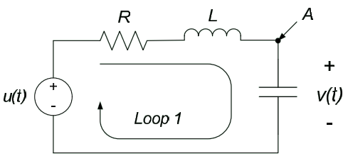
1. For the circuit shown below, apply KCL at node A and KVL around loop 1 to write two first order differential equations in two unknowns: the current through the inductor and the voltage across the capacitor. Place the two equations in state variable format.

2. Write a state variable model {A,b,c,d} for the circuit of problem 1 if the output is the voltage across the capacitor.

3. Write a state variable model {A,b,c,d} for the circuit of problem 1 if the output is the voltage across the inductor.

4. Write a state variable model {A,b,c,d} for the circuit of problem 1 if the output is the voltage across the resistor.

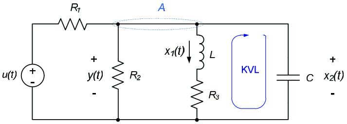
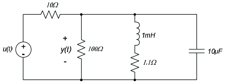
5. Write a state variable model for the circuit below. u(t) is the input voltage, and y(t) is the output. (Hint: you might want to try applying KCL at node A and KVL around the indicated loop.)

Analytical solutions of the state variable or input-output models is difficult or impossible for higher-order or nonlinear systems. Thus, numerical (or computer-based) solutions of these differential equations have become increasingly popular. This chapter provides a brief outline describing the use of some special-purpose MATLAB commands for simulating the response of linear, time invariant systems (these are systems which are governed by linear differential equations with constant coefficients).

Some MATLAB functions presented in this chapter are available in MATLAB’s Control Systems Toolbox. The Control Systems Toolbox comes with the Student Edition of MATLAB. For more information about MATLAB products, see the MathWorks web site at http://www.mathworks.com.

This section assumes some knowledge of basic MATLAB syntax. For those who are not familiar with MATLAB, a brief overview of the necessary topics is provided in Appendix A.1 of this textbook.

MATLAB’s Control Systems Toolbox contains a number of special-purpose commands for simulating the response of linear, time-invariant systems. Among these commands are commands specific to determining the step response and natural response of systems; we will restrict our attention to these commands in this chapter. Later courses in your engineering curriculum will most likely present more general-purpose MATLAB commands.

To calculate system responses (e.g. to solve the differential equations of interest), we will use only MATLAB’s step and initial commands in this chapter. The step command calculates a unit step response for the system, while the initial command calculates the natural response of a system to some set of initial conditions. We will also use the ss command to create state space model objects, to send to the step and initial commands. Basic syntax for these commands is provided below.

step: The command [y,x,t]=step(sys) returns the step response of the state variable model described by model object sys. The vector y contains the system output, the matrix x contains the states, and the vector t contains the time samples.

• The command [y,x]=step(sys) returns the step response as above, but calculated over the specified time vector t.
• The command [y,t]=step(sys) returns the system output as above, and the times at which the response is calculated, but not the state variables x.
• step(sys) with no left-hand arguments results in a plot of the step response output.

initial: Response of linear system to an initial condition. [y,x,t]=initial(sys,x0) returns the response of the system described by the model object sys to an initial condition contained in the vector x0. Variations on this command are similar to those provided above for the step command.

ss: Create a state space model object. sys = ss(A, b, c, d) returns an object named sys which provides a state space model corresponding to the matrices provided in A, b, c, and d.

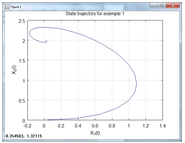
Determine and plot the response of the system of example 9.1 if $$u(t) = \begin{cases} 0V, t < 0 \\ 2V, t \geq 0 \\ \end{cases}$$

and the circuit is initially relaxed (i.e. all voltages and currents in the system are initially zero). Also plot the state trajectory for this input. The state equations for the circuit of example 9.1 were previously determined to be:

$$\begin{bmatrix} \dot{x}_1 \\ \dot{x}_2 \end{bmatrix} = \begin{bmatrix} -2 & -2 \\ 2 & 0 \\ \end{bmatrix} \begin{bmatrix} x_1 \\ x_2 \end{bmatrix} + \begin{bmatrix} 2 \\ 0 \\ \end{bmatrix} u(t)$$

While the output equation is:

$$y= \begin{bmatrix} 0 & 1 \end{bmatrix} \begin{bmatrix} x_1 \\ x_2 \end{bmatrix} + 0 \cdot u$$

Thus, the matrices describing the state space model are:

$$A= \begin{bmatrix} -2 & -2 \\ 2 & 0 \end{bmatrix}, \underline{b} = \begin{bmatrix} 2 \\ 0 \end{bmatrix}, \underline{c} = \begin{bmatrix} 0 & 1 \end{bmatrix}, d=0$$

To simulate the response of the system we first need to input the state variable model. We begin by defining the $\underline{A}$, $\underline{b}$, $\underline{c}$, and d matrices as follows:

$$ >> A = \begin{bmatrix} -2 & -2; & 2 & 0 \end{bmatrix}; \\ >> b = \begin{bmatrix} \\ 2; & 0 \end{bmatrix}; \\ >> c = \begin{bmatrix} \\ 0 & 1 \end{bmatrix}; \\ >> d = 0; $$

The » symbols denote the command prompt at MATLAB’s command window; they are included here to emphasize MATLAB commands.

It is generally desirable to create a model object in MATLAB to represent the system model⁶⁾. To create a state space system model, the command is ss. Arguments to the command are the above matrices; the output is the system model object. To create a model of our system, we type:

$$>> \text{sys = ss(A, b, c, d)};$$

Our workspace now contains a state space model object of our system named “sys”.

We can simulate the response of this system to the desired input by using MATLAB’s step command. The step command assumes that the system is initially relaxed and the input to the system is:

$$u(t) = \begin{cases} 0, t < 0 \\ 1, t \geq 0 \\ \end{cases}$$

The input to our system is exactly twice this input, so we can simply scale our output by a factor of two. (This works because the system is linear – don’t try this with a nonlinear system!) The appropriate commands are (note that we have to scale both the output and the states, since we will be plotting the output response and the state trajectory):

$$>> [y,x,t] = step(sys); \\ >> y = 2*y; \\ >> x = 2*x; \\$$

The final step is to plot the responses. Plotting the output response can be accomplished with the following commands:

$$>> \text{figure} \\ >> \text{plot}(t,y) \\ >> \text{title('System output vs. time')} \\ >> \text{xlabel('Time, sec')} \\ >> \text{ylabel('Response, Volts')} \\$$

Which results in the figure below:

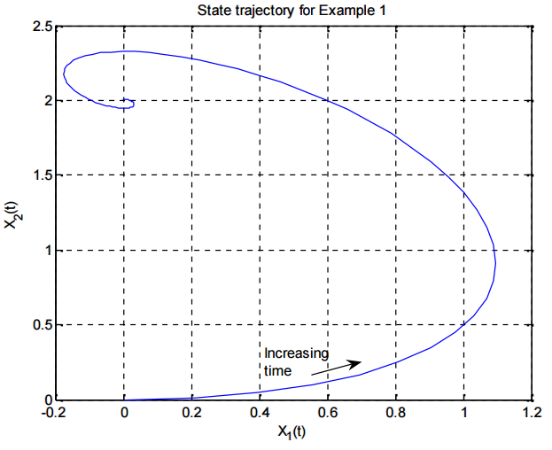
We can plot the state trajectory by plotting the second state vector, $x_1(t)$, vs. the first state vector, $x_2(t)$. MATLAB returns the first state vector as the first column of the x matrix, the second state vector as the second column of the x matrix, and so on. Thus, we can plot the state trajectory with the following commands:

$$>> \text{plot}(x(:,1),x(:,2)) \\ >> \text{grid} \\ >> \text{xlabel}('X_1(t)') \\ >> \text{ylabel}('X_2(t)') \\ >> \text{title('State trajectory for Example 1')} \\$$

• If you have access to MATLAB’s control system toolbox,
  • A state space model object can be created with the ss function. Inputs to the function are the A, b, c, and d matrices of the state space model.
  • The step command can be used to calculate the step response of the system.
  • The initial command can be used to calculate the natural response of the system.

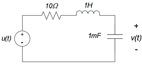
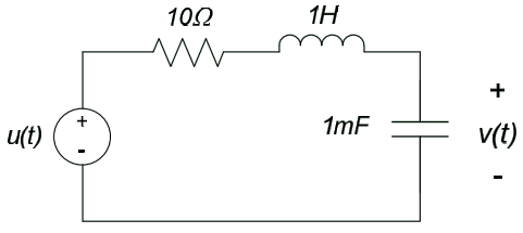
1. Simulate the response $y(t)$ of the circuit below, if $u(t)$ is a unit step function.

2. Simulate the response $y(t)$ of the circuit below, if $u(t)$ is a unit step function.

This chapter provides a brief outline describing the use of some special-purpose Octave commands for simulating the response of linear, time invariant systems (these are systems which are governed by linear differential equations with constant coefficients).

Octave is an open-source software with many of the same capabilities as MATLAB. Unlike MATLAB, however, Octave is available for free. For more information about Octave, see the web site at http://www.gnu.org/software/octave/. Octave syntax is very similar to MATLAB syntax, so the commands in this section are very similar to those provided in section 9.2.

This section assumes some knowledge of basic Octave syntax. For those who are not familiar with Octave, a brief overview of the necessary topics is provided in Appendix A.2 of this textbook.

Like MATLAB, Octave provides a number of special-purpose commands for simulating the response of linear, time-invariant systems. Among these commands are commands specific to determining the step response and natural response of systems; we will restrict our attention to these commands in this chapter.

To calculate system responses (e.g. to solve the differential equations of interest), we will use only Octave’s step and initial commands in this chapter. The step command calculates a unit step response for the system, while the initial command calculates the natural response of a system to some set of initial conditions. We will also use the ss command to create state space model objects, to send to the step and initial commands. Basic syntax for these commands is provided below.

step:

The command [y,t]=step(sys) returns the step response of the state variable model described by the model object sys. The vector y contains the system output, the matrix x contains the states, and the vector t contains the time samples.

• The command [y]=step(sys,t) returns the step response as above, but calculated over the specified time vector t.
• The command [y,t]=step(sys) returns the system output as above, and the times at which the response is calculated, but not the state variables x.
• step(sys) with no left-hand arguments results in a plot of the step response output.

initial:

Response of linear system to an initial condition. [y,x,t]=initial(sys,x0) returns the response of the system described by the state space model {A,b,c,d} to an initial condition contained in the vector x0. Variations on this command are similar to those provided above for the step command.

ss:

Create a state space model object. sys = ss(A, b, c, d) returns an object named sys which provides a state space model corresponding to the matrices provided in A, b, c, and d.

Determine and plot the response of the system of example 9.1 if

$$u(t) = \begin{cases} 0V, t < 0 \\ 2V, t \geq 0 \\ \end{cases}$$

and the circuit is initially relaxed (i.e. all voltages and currents in the system are initially zero). Also plot the state trajectory for this input. The state equations for the circuit of example 9.1 were previously determined to be:

$$\begin{bmatrix} \dot{x}_1 \\ \dot{x}_2 \end{bmatrix} = \begin{bmatrix} -2 & -2 \\ 2 & 0 \\ \end{bmatrix} \begin{bmatrix} x_1 \\ x_2 \end{bmatrix} + \begin{bmatrix} 2 \\ 0 \\ \end{bmatrix} u(t)$$

While the output equation is:

$$y= \begin{bmatrix} 0 & 1 \end{bmatrix} \begin{bmatrix} x_1 \\ x_2 \end{bmatrix} + 0 \cdot u$$

Thus, the matrices describing the state space model are:

$$A= \begin{bmatrix} -2 & -2 \\ 2 & 0 \end{bmatrix}, \underline{b} = \begin{bmatrix} 2 \\ 0 \end{bmatrix}, \underline{c} = \begin{bmatrix} 0 & 1 \end{bmatrix}, d=0$$

To simulate the response of the system we first need to input the state variable model. We begin by defining the $\underline{A}$, $\underline{b}$, $\underline{c}$, and d matrices as follows:

$$ > A = \begin{bmatrix} -2 & -2; & 2 & 0 \end{bmatrix}; \\ > b = \begin{bmatrix} \\ 2; & 0 \end{bmatrix}; \\ > c = \begin{bmatrix} \\ 0 & 1 \end{bmatrix}; \\ > d = 0; $$

The > symbols denote the command prompt at Octave’s command window; they are included here to emphasize Octave commands.

Unlike MATLAB, Octave requires you to create a model object to represent the system model. To create a state space system model, the command is ss. Arguments to the command are the above matrices; the output is the system model object. To create a model of our system, we type:

$$ > \text{sys} = ss(A, b, c, d);$$

Our workspace now contains a state space model object of our system named “sys”.

We can simulate the response of this system to the desired input by using Octave’s step command. The step command assumes that the system is initially relaxed and the input to the system is:

$$u(t) = \begin{cases} 0, t < 0 \\ 1, t \geq 0 \\ \end{cases}$$.

The input to our system is exactly twice this input, so we can simply scale our output by a factor of two. (This works because the system is linear – don’t try this with a nonlinear system!) The appropriate commands are (note that we have to scale both the output and the states, since we will be plotting the output response and the state trajectory):

$$ > [y,t] = \text{step}(sys); \\ > y = 2*y; \\ $$

The final step is to plot the response. Plotting the output response can be accomplished with the following commands:

$$ > \text{plot}(t,y) \\ > \text{title('System output vs. time')} \\ > \text{xlabel('Time, sec')} \\ > \text{ylabel('Response, Volts')} \\ $$

which results in the figure below:

In order to plot the state trajectory using Octave, we must modify our state space model somewhat. Unlike MATLAB, the states themselves are not returned by Octave’s step command. However, we can alter our c and d matrices so that the output, y, contains both system states. We will set up our output equations as follows:

$$ \begin{bmatrix} y_1(t) \\ y_2(t) = \end{bmatrix} \begin{bmatrix} 1 & 0 \\ 0 & 1 \end{bmatrix} \begin{bmatrix} x_1 \\ x_2 \end{bmatrix} + \begin{bmatrix} 0 \\ 0 \\ \end{bmatrix} u$$

This is implemented in Octave by re-setting the c and d matrices, re-calculating the model object, and re- calculating the system response with the following commands:

$$ > c = [1 0; 0 1]; \\ > d = [0; 0]; \\ > sys = ss(A,b,c,d); \\ > [y,t] = \text{step}(sys); \\ > y = 2*y; $$

Now, the output $y_1(t)$ is simply the state $x_1(t)$ and the output $y_2(t)$ is the state $x_2(t)$. Octave returns the first state vector as the first row of the y matrix, and the second state vector as the second row of the y matrix. Thus, we can plot the state trajectory with the following commands:

$$ > \text{plot}(y(1,:),y(:,2)) \\ > \text{grid} \\ > \text{xlabel}('X_1(t)') \\ > \text{ylabel}('X_2(t)') \\ > \text{title('State trajectory for Example 1')} $$

• Octave allows you to simulate linear, time invariant systems with the following commands:
  • A state space model object can be created with the ss function. Inputs to the function are the A, b, c, and d matrices of the state space model.
  • The step command can be used to calculate the step response of the system.
  • The initial command can be used to calculate the natural response of the system.

1. Simulate the response $y(t)$ of the circuit below, if $u(t)$ is a unit step function.

2. Simulate the response $y(t)$ of the circuit below, if $u(t)$ is a unit step function.

Back to Chapter 8 Go to Chapter 10